
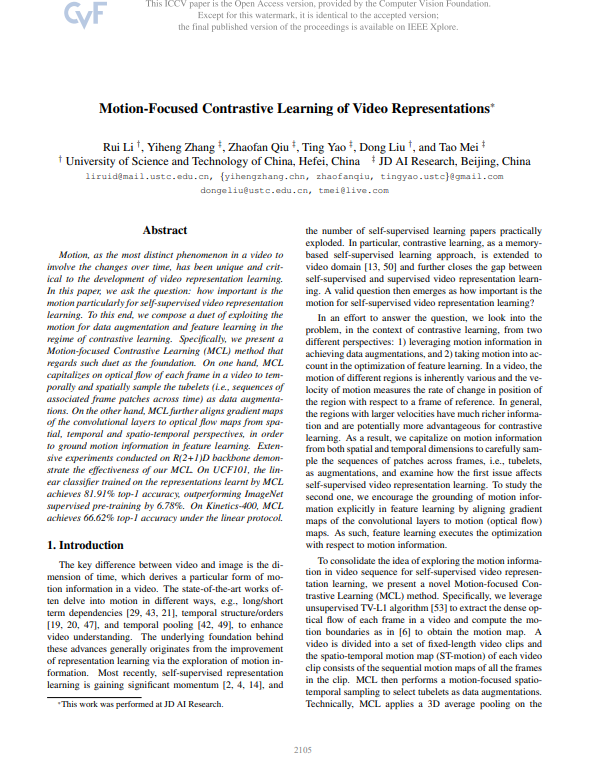
오늘 소개 드릴 논문은 Video Representation을 위해 Motion 정보에 초점을 맞춘 “Motion-Focused Contrastive Learning of Video Representation” 이라는 논문 입니다. 기존 여러 Video Representation 연구들에서는 self-supervised 방식으로 비디오를 잘 표현하기 위해, motion의 long/short term dependency 혹은 temporal order와 같이 각자의 방식으로 motion을 활용해 좋은 성능을 보여왔습니다.
본 논문의 저자는 이처럼 비디오 하면 빼놓을 수 없는 motion 정보의 magnitude가 큰 곳일 수록 비디오에서 유용한 정보를 나타내는 곳이라 판단하였고, 이것이 self-supervised video representation에 얼마나 중요한지에 대해 증명하기 위해 data augmentation 관점과 feature learning 관점에서 접근해 Motion-focused Contrastive Learning (MCL)을 제안하였습니다. 자세한 내용은 아래서 소개드리겠습니다.
1. Method
1.1 Motion Estimation
Motion을 활용하기에 앞서, 비디오에서 motion을 추정해냅니다. 우선 한 비디오 내에서 TV-L1이라는 알고리즘을 통해 optical flow를 계산해냅니다. 계산된 optical flow는 (u_i, v_i)로 2차원의 map 형태를 나타내며, 이는 pixel-level에서 그 다음 프레임과의 수평, 수직 변위를 의미합니다.
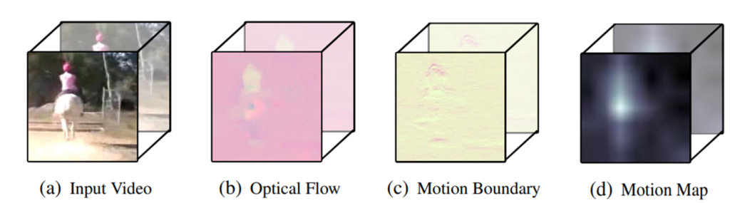
주로 이렇게 계산된 optical flow 자체를 motion으로 사용하기는 하지만, 이 optical flow에는 한가지 단점이 존재합니다. 바로 카메라의 움직임이 고려되지 않았다는 점으로, 이 때문에 실제로는 정적인 scene 혹은 object 이지만 촬영하는 camera가 움직여 optical flow에서 높은 magnitude를 보인다는 것입니다. 그러나, 비디오를 통해 표현하고자 하는 것은 실제 상황에서 움직임이 큰 instance가 주를 이루기 때문에 optical flow map에서 camera motion을 제거해야만 실제 motion 정보를 획득할 수 있습니다.
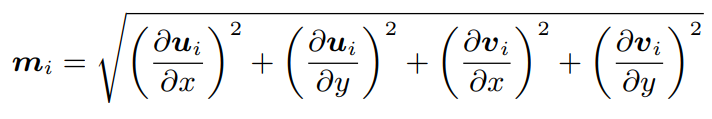
이 같은 목적으로 optical flow map에서 다른 연구에서 제안되었던 motion boundary 방식(optical flow map의 각 원소를 x, y 축으로 편미분)을 도입하였습니다. Camera motion을 제거하는 방식은 이러한 motion boundary에서 magnitude를 구하는 것으로 식 (1)과 같이 계산되며, 결과적으로 2차원의 motion map m_i가 생성됩니다. Fig 3에서 볼 수 있듯이, motion map이 실제로 움직임이 있는 instance를 잘 포착하는 것을 알 수 있습니다.
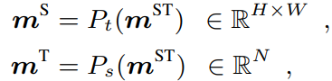
이렇게 생성된 motion map을 각 프레임마다 만들고, 한 비디오에 대하여 총 세 종류의 pre-define된 형태로 생성하였습니다. 이들은 모든 프레임에서 나온 motion map을 stack한 형태로 NxHxW 크기의 ST-motion m^{ST}, 그리고 식 (2)처럼 각각 temporal dimension과 spatial dimension으로 average pooling한 S-motion m^{S}과 T-motion m^{T} 입니다.
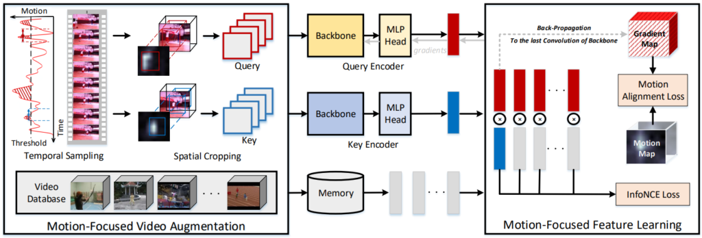
1.2 Motion-Focused Video Augmentation
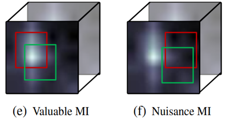
Self-supervised feature representation 연구들에서는 한 instance에 대한 서로 다른 두 view 간의 거리를 좁히는 contrastive learning 방식을 활용해 feature의 generality를 높입니다. 또한, 한 연구에서는 이에 대한 generality를 boost 하기 위해서는 불필요한 nuisance 정보를 제거하고 task-relevant한 정보만을 포함한 mutual information이 필수적이라는 것을 밝혀냈습니다. 이때, 비디오 관련 연구에서 motion은 결국 video-represenation과 관련된 task-relevant한 정보입니다. 그러므로 Fig 4의 (e)처럼 motion 정보에만 초점을 맞추는 것이 generality를 boost 할 수 있는 방법이며, 이러한 논지에 따라 본 논문에서 저자는 두 단계의 motion-focused video augmentation을 제안하였습니다.
먼저, 두 단계 중 첫번째로 temporal sampling 과정을 거칩니다. Temporal sampling 과정은 한 비디오를 여러 개의 clip으로 나누고, 각 clip 마다의 T-motion m^{T}을 계산합니다. 이후, 모든 clip에 대해 m^{T} 평균의 median을 threshold로 두고 이 값 이상인 clip을 랜덤 샘플링해 positive pair로 선택합니다.
이후, spatial cropping 과정도 거칩니다. 이 과정에서는 앞서 선택한 두 clip에서 각각 S-motion m^{S} 을 계산하고, 이 motion map에서 90분위수를 threshold로 선정합니다. 그리고, threshold보다 높은 값을 가지는 pixel을 80퍼센트 이상 포함하도록 bounding box를 생성하고, 각 clip에 대해 그 영역을 crop 하게 됩니다. 이후, crop된 영역에 color-jittering, random scales, grayscale, blur, mirror와 같은 변환을 적용하였습니다.
1.3 Motion-Focused Feature Learning
앞서 언급한대로, motion은 비디오 task-relevant한 정보임으로 augmentation 뿐만 아니라 feature learning 관점에서도 boosting 시킬 수 있습니다. 이를 위해 본 논문에서는 motion alignment loss (MAL)을 제안하였습니다. MAL은 convolution layer에서 생성된 feature map 혹은 gradient map에 motion map을 적용하여 motion이 존재하는 위치를 focusing 하는 방식으로 motion-guided한 attention이라고 생각하시면 될 것 같습니다. 이 같은 MAL은 적용 방식에 따라 세 종류로 나뉩니다.
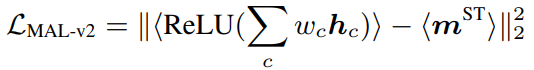
먼저, “alignment feature map” 방식은 motion이 큰 부분은 feature map에서 high response가 되도록 기대하고, 식 (3)과 같이 feature map을 channel 축으로 합한 값의 normalize map과 motion map이 normalize 된 것 간의 loss로 설계된 방식입니다. 여기서 <>는 L2 normalize, c는 channel 축으로의 인덱스를 의미합니다.
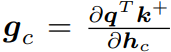
다음으로, “align weighted feature map” 방식은 GradCAM에서 영감을 받아, 식 (4)와 같이 feature map에 gradient weight를 준 방식 입니다. Gradient weight w_c는 gradient map g_c의 평균으로 계산되며, g_c는 식 (5)와 같이 계산 됩니다. 이때 q와 k^{+}는 각각 query와 key (두개의 view) 들의 feature vector를 의미합니다.
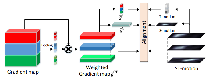
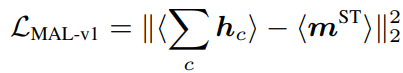
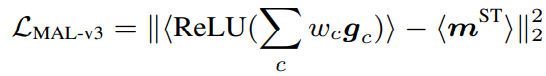
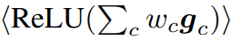
마지막으로, “Align weighted gradient map” 방식은 model이 weight를 update할 때 직접적으로 guide해줄 수 있도록, 이전 형태에서 feature map을 gradient map으로 대체한 식 (6)과 같은 형태 입니다. 추후에 언급하겠으나 해당 형태가 가장 성능이 높아 default motion alignment loss로 선정되었습니다.
그리고, 위의 세 형태에서는 ST-motion m^{ST} 활용하여 동시에 처리하였기에, 좀더 temporal 혹은 spatial axis 각각에 초점을 맞출 수 있도록 S-motion 혹은 T-motion만을 활용한 loss term도 추가하였습니다. 이를 통해 식 (7)과 같은 형태로 최종적인 MAL Loss가 설계되었습니다. 여기서 \bar{g}는 식 (8)과 같은 것으로 motion map만 위첨자에 맞게 바뀌는 형태 입니다.

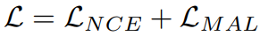
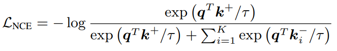
이러한 MAL Loss와 기존 contrastive learning에서 자주 사용하는 NCE Loss를 더한 형태를 식 (9)와 같이 학습을 위한 최종적인 Loss 형태로 두고 학습하게됩니다. 식 (10)은 NCE Loss를 나타내며 q와 k^{+}는 두 개의 view에서 나온 vector, 즉 positive 관계를 나타내며, k^{-}는 negative 관계인 K개의 feature를 나타냅니다.
2. Experiments
2.1 Ablation Study
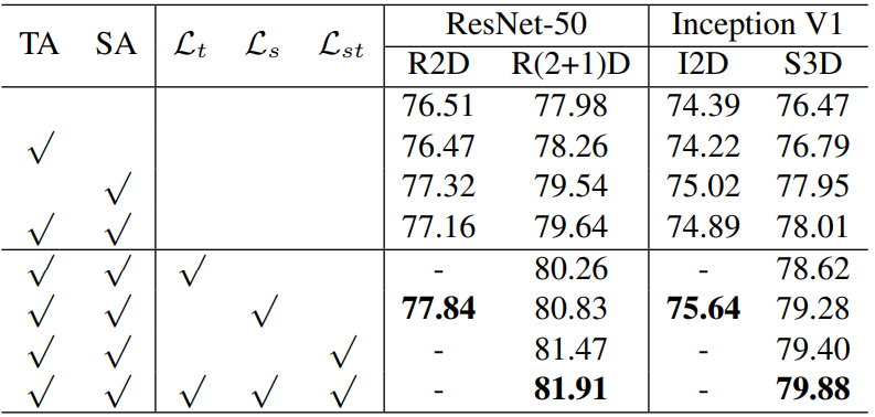
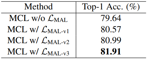
Table 1은 MCL의 component에 대한 ablation study 입니다. Motion-Focused Video Augmentation에 해당하는 TA는 temporal sampling, SA는 spatial cropping을 의미하며, 중간 L_{t}, L_{s}, L_{st}는 Motion-Focused Feature Learning을 위해 설계된 식 (7)에서 합해진 세 항을 의미합니다. 또한 다양한 backbone에 대한 성능도 들어있으며, 신기한건 2D backbone network에 대한 성능도 포함되어 있습니다. Table 1을 통해, motion에 초점을 두어 제안된 두 가지 방식 모두 하나의 element를 추가함에 따라 성능이 오르는 경향을 보였으며, 특히 L_{st}의 경우 해당 element를 하나 추가하는 것만으로 1.5퍼센트 정도의 가장 높은 효력을 보였습니다.
Table 2는 MAL Loss의 형태에 따른 ablation study로, 왜 세번째 형태가 default가 되었는지를 알 수 있습니다.
2.2 Evaluations on Linear Protocol
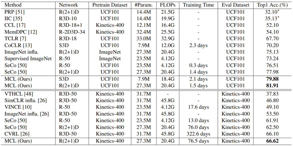
Table 3는 MCL 방식으로 학습된 backbone network의 표현력을 평가한 결과입니다. 모델에 classifier를 붙여 classification한 것이 아닌, scratch-level에서 학습된 feature로 SVM을 학습해 성능 평가한 방식으로 feature 자체의 표현력을 비교할 수 있습니다. UCF101과 Kinetics-400에서 모두 가장 높은 성능으로 SOTA를 달성하였고, 같은 backbone인 기존 SOTA와 비교했을 때 2퍼~4퍼 정도의 높은 향상을 보였습니다.
2.3 Evaluations on Downstream Tasks
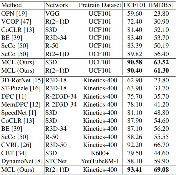
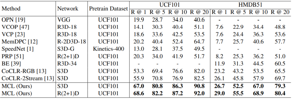
Table 4와 5는 각각 MCL로 pretrain된 backbone network를 downstream task인 action recogntion과 video retrieval에 적용한 결과 입니다. 모든 downstream task에서 높은 성능 차이로 SOTA를 달성하였습니다.
2.4 Visualizing Self-supervised Representation
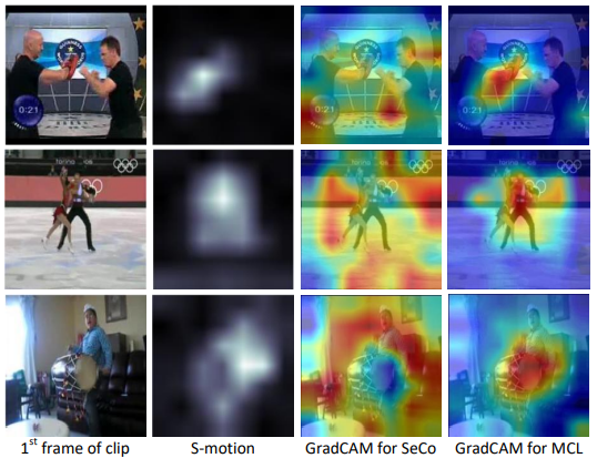
Fig 6은 기존 SOTA였던 SeCo와 제안된 MCL 간의 Grad-CAM을 비교한 정성적 결과 입니다. 실제로 instance의 motion이 나타난 위치를 MCL이 더 잘 포착하는 것을 보실 수 있습니다.
3. Reference
[1] https://openaccess.thecvf.com/content/ICCV2021/papers/Li_Motion-Focused_Contrastive_Learning_of_Video_Representations_ICCV_2021_paper.pdf