[AAAI 2021] BSN++ : Complementary Boundary Regressor with Scale-Balanced Relation Modeling for Temporal Action Proposal Generation

바로 이전에, Temporal action proposal 생성하는 BSN (Boundary Sensitive Network)에 대해 리뷰 했었습니다. 이번에 리뷰할 BSN ++ 은, BSN 의 상위 버전인 네트워크라고 생각하면 될 것 같습니다. (저자도 겹칩니다…!) 그렇기 때문에, BSN 에서 있었던 단점을 극복하는 방식으로 3가지의 기여를 했습니다.

기존의 BSN 은 flexible 한 durations 와 reliable 한 confidence scores 를 가진 proposals 를 생성한다는 장점이 있었습니다. 그러나, 3가지 단점이 존재합니다.

1. boundary 를 예측할 때, 해당 boudnary 근처의 local deatils 만 사용합니다. 즉, 전체적인 video sequence 에 있는 temporal contexts 를 사용하지 않았습니다.
2. confidence 를 평가할 때, proposal 과 proposal 간의 relation 을 고려하지 않았습니다.
3. positive/negative proposals 와 temporal durations 의 imbalance data distribution 도 고려하지 않았습니다.

BSN 의 이런 문제들을 해결하는 temporal proposal generation 을 위해, 본 논문에서는 BSN ++ 을 제안합니다. 위에 있는 단점들과 매칭되는, 해결방법들에 대한 간략한 소개입니다.

1. boundary prediction 할 때 rich contexts 를 사용하기 위해, U-shaped architecture 와 nested skip connection 을 사용합니다.

이렇게 하면, 두 개의 최적화된 boundary classifiers 가 ‘같은 목표’ (background → action 이나 action → background 변화를 detect 하는 것 : starting, ending 을 의미) 를 공유하게 돼서, 서로 상호보완을 해줄 수 있습니다. 그리고 이 상태에서, complementary boundary regressor 라는 것을 도입합니다. 왜냐면, input videos 를 역방향으로 가공하면, starting classifer 로 ending locations 를 predict 하는데에도 쓸 수 있기 때문입니다. (그 반대도 마찬가지) 이렇게 하면 추가적인 parameter 없이도 높은 precision 을 달성할 수 있습니다.

2. densely- distributed proposals 의 confidence scores 를 predict 하기 위해, proposal-proposal relation modeling 에서 channel-wise / position-wise global dependencies 를 둘 다 고려하는 a proposal relation block 을 디자인했습니다.

3. sampling postivies / negatives 간의 imbalance scale-distribution 를 완화시키기 위해, IoUbalanced (positive-negative) sampling 과 scale-balanced re-sampling 으로 구성되어 있는 a two-stage re-sampling sheme 를 구현했습니다.

또한 BSN++ 은, boundary map 과 confidence map 이 a unified framework 에서 동시에 생성되고, 결합되어 trained 됩니다. (BSN 은 unified 아님!)

즉, 본 논문에서는 기존 BSN 의 문제들을 해결하는 temporal proposal generation 을 생성할 수 있는, BSN++ 을 제안합니다.

Our Approach

Problem Definition

an untrimmed video sequence : U = \{u_t\}^{l_v}_{t=1}

• u_t : 길이가 l_v 인 video 의 t 번째 frame

A set of action instances : \psi_g =\{ \phi_n = (t^s_n , t^e_n ) \}^{N_g}_{n=1}

• Video S_v 에서 temporally annotated 된 action instances 이다.
• N_g 는 ground truth action instances 의 수 이다.
• t^s_n, t^e_n 는 각각 n 번째 action instance \phi_n 의 starting time, ending time 이다. (training phase 에서 제공된다.)
• testing phase 에서, 우리가 예측한 predicted porposal set \psi_p 가 \psi_g 를 high recall / high temporal overlapping 으로 cover 해야 한다.

Video Feature Encoding

BSN++ 을 적용하기 전에, 우선 Two-stream networks 를 사용해서 visual features 를 encode 합니다.

아무래도 비디오의 길이가 길면 computational cost 가 커지니까, l_v 개의 frames 를 가진 하나의 untrimmed video S_v 를, interval \sigma 을 이용해서 가공합니다. 또한 해당 network 의 마지막 FC layer 의 output 을 concat 해서, F = \{f_i\}^{l_s}_{i=1} 로 만듭니다. 이때 l_s = l_v / \sigma 입니다. 이 feature sequence F 가 BSN ++ 의 입력으로 사용되는 것입니다.

Proposed Network Architecture : BSN++

BSN 은 여러 개의 stages 로 이루어져 있었는데, BSN++ 은 proposal map을 하나의 network 에서 만들어냅니다.

BSN++ 은, boundary information 을 나타내는 boundary map 과, densely distributed proposals 의 confidence scroes 를 나타내는 confidence map 을 생성하도록 디자인 됐습니다. 이때, BSN++ 은 세 개의 modules 로 이루어져 있습니다.

• Base Module : input video featurse 를 이용해서, temproal information modeling 을 수행한다. (output features 가 이후 두 모듈에서 사용된다)
• Complementary Boundary Generator : a nested U-shaped encoder-decoder 를 사용해서, input video features 를 가공해서 boundary probabilities sequence 를 평가한다.
• Proposal Relation Block : 서로 complementary dependencies 가 있는, 두 개의 self-attention modules 를 사용해서, proposal-proposal relations 를 model 한다.

Base module

temporal relation modeling 을 할 수 있는 features 를 extract 하는 모듈입니다. 해당 모듈에는 두 개의 1d convolutional layers (256 filters, kernel size 3, stride 1) + ReLU activation layer 가 있습니다. 이 모듈에서 extracted 된 features 는 이후에 두 모듈의 input 으로 들어갑니다. (이 때, video 의 길이는 정해지지 않았기 때문에, 일련의 sliding windows로 video sequence 를 잘라냅니다)

Complementary Boundary Generator

image segmentation 에서 성공적으로 쓰였던 U-net 에 영감을 받아서 디자인 됐습니다. Encoder-Decoder networks 는 high-level 의 global context 와 low-level 의 local details 를 동시에 잘 포착한다는 특징을 가집니다.

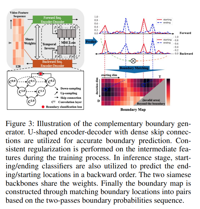
해당 그림 에서, 각 원은 1D convolutional layer ( 512 filters, kernel size 3, stride 1) + batch normalizatoin layer + ReLU layer 를 나타냅니다.

1. 두 개의 down-sampling layers 를 추가해서 receptive fields 를 확장시키고, 두 개의 up-sampling layers 를 추가해서 origianl temporal resolution 을 회복 시킨다 → overfitting 방지
2. 빨간 점 : deep supervision → fast convergent speed 를 위해 수행됨
3. nested skip connections → decoder 와 encode 의 feature maps 을 fusion 하기 전에, semantic gap 을 bridgin 하기 위해 적용됨

starting classifier : background to actions 와, actions to background 의 순간적인 변화를 detect 하도록 학습됩니다.

따라서, input video 를 거꾸로 된 상태로 가공시킨다면, starting classifer 는 pseudo ending classifier 로 고려될 수 있기 때문에, bi-directional prediction results 는 상호보완적이 되는 것입니다. 덕분에 bidirectional encoder-decoder networks 는 parallel 하게 optimized 됩니다. 그리고, prediction layer 전에, consistent constraint ( f(x^f), f(x^b) 부분) 으로 regularization 이 forward / backward 모두의 intermediate features 에 적용됩니다.

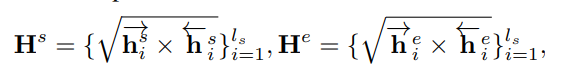
inference stage (새로운 입력 데이터를, training 을 통해 만들어진 모델에 넣어서 결과를 내놓는 과정) 에서, encoder-decoder network 가 적용되어서, starting heat map \vec{ H^s} = {\vec{h^s_i}^{l_s}{i=1} 와 ending heat map \vec{H^e} = {\vec{h^e_i}^{l_s}{i=1} 를 예측합니다. 이때, h^s_i 와 h^e_i 는 각각 i-th snippet 의 starting 확률과 ending 확률을 나타냅니다. (이 부분이랑 바로 아래 쪽… 해결 방법 못 찾은… 그치만 언젠가 넣고 싶어서 당분간 이렇게 두겠습니다…!)

input feature sequence 를 거꾸로 된 순서로 만들어서, 동일한 backbone 에 넣습니다. 마찬가지로 starting heat map 과 ending heat map 을 얻는데, 이때 벡터 표시는 반대입니다. 이 두 과정 후에, 높은 scores 를 가진 boundaries 를 선택하기 위해, 두 쌍의 heatmaps 를 fuse 해서, final heat map 을 얻습니다.

이 두 개의 boundary points heatmaps 를 이용하면, boundary map M^b \in R^{1 \times D \times T} 를 만들 수 있습니다. 이건, 모든 densely distributed proposals 의 boundary information 을 나타냅니다. 이때 T 는 feature sequence 의 길이이고, D 는 proposals 의 maximum duration 입니다.

M^b_{j,i} = /{/{h^s_i \times h^e_{i+j| /}^T_{i=1}/}^D_{j=1}, i+j < T,

Proposal Relation Block

이 모듈의 목표는, dense proposals 의 confidence scores 를 평가하는 것입니다. BMN 의 방법을 따라서, proposal feature map F^p \in R^{D \times T \times 127 \times N} 를 생성합니다. (이때 N = 32) 이 feature map 이 하나의 3D convolutional alyer (kernel size 1 x 1 x 32, 512 filters) + ReLU 에 태워집니다. 따라서, reduced proposal feature maps 는 \widehat{F^p} \in R^{D \times T \times 512} 입니다.

proposal relation block 은 두 개의 self-attention modules 로 이루어져 있습니다.

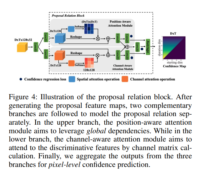
Proposal realtion block (1) : Position-aware attention block

proposal features maps \widehat{F^p} 를 a convolutional layer 에 따로 넣어서, 두 개의 새로운 feature maps, A 와 B 를 얻습니다. 이건 reshape / tranpose operatoins 와 함께 spatial matrix multiplcation 을 적용하기 위함입니다.

그 이후에, 이 A, B 를 이용해서, Softmax layer 가 position-aware attention P^A \in R^{L \times L} 를 계산합니다. 이때 L = D \times T

P^A_{j,i} = {{exp(A_i \dot B_j)} \over {\Sigma^L_{i=1} exp(A_i \dot B_j)}}

이때 P^A_{j,i} 는 j-th position 의 i-th attention 입니다.

마지막으로, attended features 가 proposal features 에 weighted summed 돼서, confidence 를 prediction 를 위해 convolutional layers 에 실립니다.

Proposal relation block (2) : Channel-aware attention module

이 모듈은 different channels 간의 inter-dependencies 를 이용하기 위해, channel-wise matrix multiplication 을 바로 수행합니다. 이렇게 하면, confidence prediction 할 때 쓰이는 proposal feature representatinos 를 향상시킬 수 있습니다. attention calculation 는 position aware attention block과 동일합니다. (attended dimension 만 다름) 비슷하게, proposal featurse 와 weighted summed 된 attended features 가, 이후에 2D convolutonaly layer 에서 캡쳐돼서 confidence map 을 생성합니다. 이때 confidence map 은 M^c \in R^{D \times T}

Proposal relation block의 두 attention modules 에서 나온 outputs 를 aggregate 해서, proposal confidence prediction 에 사용합니다. 마지막으로, 더 좋은 성능을 위해, 세 개의 브랜치에서 나온 predicted confidence maps 를 fuse 합니다.

Re-sampling

데이터 분산 불균형이, 특히 long-tailed dataset 에서는, 모델 학습에 악영향을 줄 수 있습니다. 따라서 positive/negative samples distribution 을 고려해서, confidence prediction 의 성능을 향상시키고, proposal-level resampling method 를 디자인해서, long-tailed dataset 에서의 학습 성능을 높이고자 합니다.

해당 논문에서 resampling 전략은 두 개의 stages 로 구성되어 있습니다. 이는 positives / negatives proposals 를 균형있게 하는 것 뿐만 아니라, proposals 의 temporal duration 또한 균형있게 합니다.

IoU sampling

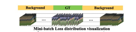
해당 논문의 티저 이미지를 보면, mini-batch loss distirubtion 에서, positives 와 negatives 가 많이 차이 나는 것을 볼 수 있습니다. 이는 training model 을 편향되게 만들 것이기 때문에, 이걸 균형있게 할 수 있는 방법을 고안해야 합니다.

Scaled-balanced re-sampling

long-tailed scales 에서 이 이슈를 완화시키기 위해, 우리는 2-stage positive/negative re-sampling method 를 제안한다. 이는 IoU-balanced sampling 방법을 따릅니다.

P_i 는, scale s_i 의 positive proposals 의 수 이고, r_i 는 s_i 의 positive 비율이므로, {P_i} \over {\Sigma^{N_s}_{j=1} P_j } 입니다. N_s 는, pre-defined normalized scale regions 의 수 입니다.

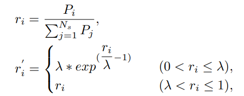
positive ration sampilng function 을 디자인해서, r_i 에 따른 resulting ratio r_i ‘ 를 얻을 수 있습니다. 따라서, re-normalized 된 r_i ‘ 를, 특정 proposal scale region s_i 에 sampling probability 로 사용해서 mini-batch data 를 만듭니다. negative proposals 에 대해서도 동일한 과정이 수행됩니다.

Training and Inference of BSN++

Training : 데이터를 이용해서, weight 를 업데이트 하여 모델을 만드는 과정

Training : Overall objective function.

L_{BSN++} = L_{CBG} + \beta \dot L_{PRB} + \gamma \dot L_2(\theta)

CBG : complementary boundary generator

PRB : proposal relation block

L1 는 regularization iterm 이고, 베타랑 감마는 두 모듈 간의 trade-off 를 조절하고, overfitting 을 완화하기 위함입니다.

Training : Data

길이 l_s 짜리 extracted feature F 를 sliding windows 를 이용해서 잘라서, 75% temporal overlapping 이 있는, 길이 l_w 짜리로 만듭니다.

그리고 그걸로 training dataset \Phi = \{F^w_n\}^{N_w}_{n=1} 를 만듭니다. 이때 N_w 는 최소 하나의 ground-truth 를 포함하는 retained windows 의 개수입니다.

Training : Label Assignment

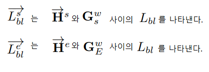
Complementary Boundary Generator (CBG)에서, boundary probabilities sequence 를 predict 하기 위해, 상응하는 label sequence G^w_s , G^w_e 를 만들어야 합니다.

annotation set \Psi^w_g 에 있는 각 action instacne \psi_g 에 대해, starting regions 와 ending regions 를 [t^s_g - d_{\psi} / 10, t^s_g + d_{\psi} / 10 \ 와 [t^e_g - d_{\psi} / 10, t^e_g + d_{\psi} / 10 \ 로 정의했습니다. 이때, d_{\psi} = t^e_g - t^s_g 이고, 이건 \psi_g 의 duration 입니다.

어떤 action instances 의 starting / ending regions 에 속해있는 각 temporal location 는 그에 상응하는 라벨 g^s / g^e 는 1로 설정됩니다.

따라서, CBG 에서 사용되는 starting / ending label sequence 는 각각 아래와 같습니다.

G^w_s = \{g^s_i\}^{l_w}_{i=1}, G^w_e = \{g^e_i\}^{l_w}_{i=1}

Proposal Relation Block (PRB) 에서, 우리는 모든 densely distributed proposals 에 대해 confidence map M^c \in R^{D \times l_w} 를 예측합니다.

이때, label confidence map

M^c_g = \{\{g^c_{j,i}\}^{l_w}_{i=1}\}^D_{j=1}

에 속해있는 point g^c_{j,i} 는,

\Psi^w_g 에 있는 모든 \psi_g 에 대한 proposal \psi_{j,i} = [t_s = i, t_e = i+j] 의 maximum IoU values 를 나타냅니다.

Objective of CBG

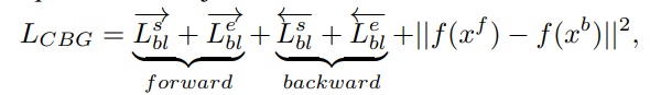
output probability 와 corresponding label sequence 간의 weighted binary logistic regression loss L_{bl} 를 objective 로 설정했습니다.

Mean-square loss 도 two-passes imtermediate features 에 대해 행해진다.

Objective of PRB.

proposal feature maps F^p 를 input 으로 받아서, PRB 는 모든 densely distributed proposals 에 대한 두 가지 confidence maps M^{cr}, M^{cc} 를 생성합니다. 이때, regression loss 와 binary classification loss 의 합으로 training objective 가 정의됩니다.

L_{PRB} = L_{reg} + L_{cls}

이전에 진행했던 two-stage sampling 에 의해, 이 시점에서의 positives 와 negatives 의 scale 과 number ratio 는 1:1 에 가깝게 되도록 보장된다고 합니다.

Inference : 새로운 입력 데이터를, training 을 통해 만들어진 모델에 넣어서 결과를 내놓는 과정

bidirectional boundary probabilities ( H^s, H^e ) 와 confidence map ( M^{cc}, M^{cr} 를 이용해서, BSN++ 이 boundary map M^b 를 생성할 수 있습니다.

이때, M^b, M^c 를 dot multiplication 해서 합쳐서, proposal map M^p 를 생성합니다.

그리고, M^p 에서 high scores 를 가진 points 를 걸러내서, post-processing 을 위한 candidate proposals 로 사용할 수 있습니다.

Score Fusion

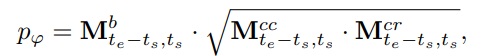
M^p 에 있는 proposals 의 final scores 는 boundary information 과 global confidence scores 에 연관되어 있습니다.

proposal \phi = [t_s, t_e] 를 예시로 했을 때, 이에 대한 final score p_{\phi} :

Redundant Proposals Suppression.

BSN ++ 이 생성하는 proposal candidate set :

\Psi = \{ \psi_n = (t_s, t_e, p_{\psi})\}^{N_p}_{n=1} , 이때 N_p 는 proposals 의 수.

생성된 proposals 가 서로 overlap 되기 때문에, Soft-NMS 알고리즘을 적용해서, redundant proposals 의 confidence scores 를 suppress 합니다.

최종 proposals set :

\Psi^{’}_p = \{ \psi^{’}_n = (t_s, t_e, p^{’}_{\psi})\}^{N_p}_{n=1}

이때 p’_{\phi} 는 decayed score 입니다.

Experiments

Datasets :

ActivityNet-1.3 : action recognition 과 temporal action detection tasks 에 쓰이는 large-scale video datasets. 19,994 개의 비디오, 200 개의 action classes.

THUMOS-14 : untrimmed videos with temporal annotations of 20 action classses.

Implementation details :

feature encoding : two-stream network (ResNet, BN-Incdeption 이 spatial and temporal networks 로 각각 사용됨)

interval \sigma : ActivityNet-1.3 에서는 16, THUMOS14 에서는 5

ActivityNet)

(1) input videos 의 feature sequence 를, linear interpolation 을 이용해서, l_w = 100 로 rescale 함.

(2) maximum duration D = 100 ( 모든 action instances 를 커버하기 위함)

THUMOS14)

(1) input videos 의 feature sequence 를, linear interpolation 을 이용해서, l_w = 128 로 rescale 함.

(2) maximum duration D = 64 ( 98%의 action instances 를 커버하기 위함)

두 데이터 셋 모두, BSN++ 을 바닥부터 학습시킨다.( optimizer = Adam, batch_size = 6, 초기 7 epoch 동안 lr = 0.001 , 이후 3 epoch 동안 lr = 0.0001)

Temporal Proposal Generation

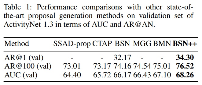
ActivityNet-1.3 에 대한 결과 비교.

BSN++ 이, sota proposal generation methods 를 큰 차이로 넘겼습니다.

AR : Average Recall

AN : Average Number

AUC : Union under AR vs. AN curve (AN ranges from 0 to 100)

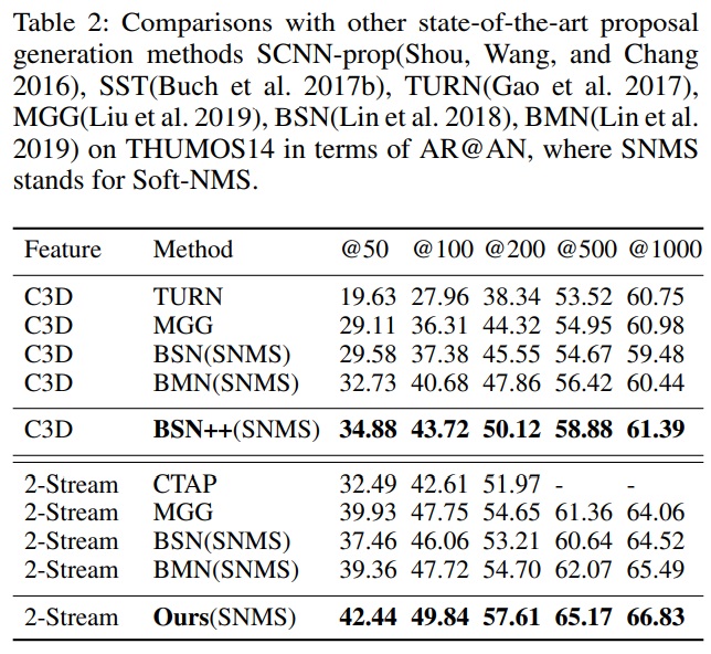
THUMOS14 에 대한 결과 비교.

featurse 는, two-stream featrues 와 C3D featurse 를 사용했습니다.

(1) 어떤 feature 를 사용하든 간에, BSN ++ 이 sota 를 달성했습니다.

(2) Soft-NMS 로 post-processed 됐을 때, 더 적은 수의 proposals 를 사용하여 더 higher 한 AR 을 얻을 수 있었습니다.

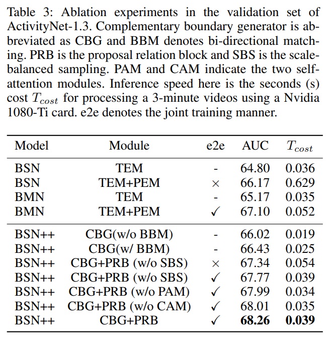
Ablation Experiments.

BSN++ 를 ActivityNet-1.3 의 validation set 을 이용하여 평가했습니다.

(1) Encoder-Decoder 구조가, accurate boundary prediction 를 위한 “local to global” context 를 효과적으로 학습했다. (이전의 works 는 local details 만 봤다)

(2) bidirectional matching mechanism 은 boundary 를 판단하는 데 있어서 중요하다는 것이 검증됐다.

(3) proposal relation block 은 accurate 하고 discriminative 한 proposals scoring 을 위한 comprehensive features 를 제공한다. (이전의 works 는 proposals 를 각각 따로 다뤘다.)

(4) scale-blanced sampling → model이 equivalent balancing 을 얻었다.

(5) separated modules 를 end-to-end netowrk 로 합침으로써, 성능 향상이 이뤄졌다.

(6) BSN++ 이 이전의 methods 에 비해, overall efficeinct 하다.

TEM : boundary probabilities sequence generation 에 local details 만 봤었습니다. 그렇지만, temporal context 를 전부 사용하지 않으면, 복잡한 시나리오에서 robust 하지 않게 됩니다. 따라서, BSN은 confidence regression 에서 proposal relations 를 model 하는 것을 실패했습니다. 또한 proposal duration 에 대한 imbalance data distribution 도 무시했습니다. 그러나, BSN++ 은 이러한 이슈들을 잘 다뤘음을 보여줍니다.

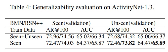
Generalizability of proposals :

두 가지 un-overlapped action subsets 를 seen 과 unseen subset 으로 선택했다고 해봅시다. Sports-1M dataset 으로 pre-trained 된 C3D network 로 featur extraction 을 하고, BSN++ 를 seen, seen+unseen training video 로 학습 시켰을 때, 해당 모델들을 validation videos 로 평가해본 결과입니다.

unseen 에서 아주 약간의 drop 만이 있었는데, 이는 BSN++ 이 great generalizability 를 갖고 있음을 뜻합니다. 따라서, unseen actions 에 대해서도 양질의 proposals 를 생성할 수 있음을 보여줍니다.

Action detection with our proposals

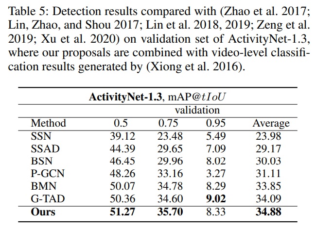
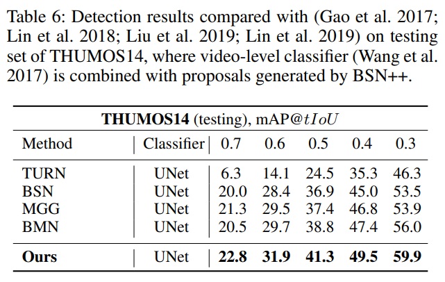
ActivityNet-1.3, THUMOS14 에서, BSN++ 이 sota 를 달성했음을 보여줍니다.

결론

temporal action proposal generation 을 위한, BSN++ 을 제안했습니다.

앞서 언급했듯 BSN 의 단점이 3가지 있었는데, 그걸 아래 3가지로 해결합니다.

complementary boundary generator

• U-shaped architecture, bi-directionnal boundary matching mechanism → boundary prediction 을 위한 rich contexts 를 학습

proposal relation block

• confidence evaluation 을 위한, proposal-proposal relations 를 model 하기 위함.
• two self-attention modules → global and inter-dependencies modeling 을 perform 함.

imbalanced data distribution of proposal duration 을 고려

• IoUbalanced (positive-negative) sampling 과 scale-balanced re-sampling 으로 구성되어 있는 a two-stage re-sampling sheme 를 구현

또한 boundary map 과 confidence map 이 하나의 network 에서, 동시에 생성됐고, ActivityNet-1.3 과 THUMOS14 에 대한 실험이 수행함으로써 temporal action proposal / detection 에서 BSN++ 이 sota 라는 것을 보여주었습니다.

논문 링크

BSN++: Complementary Boundary Regressor with Scale-Balanced Relation Modeling for Temporal Action Proposal Generation