
지난번에 리뷰 중, Video classification task에 transformer 구조를 처음 도입한 Facebook 의 TimeSformer가 2021년 2월 9일에 나왔다면 조금 지난 2021년 3월 29일 Google에서도 Video classification task에 transformer 구조를 도입한 ViViT(A Vision Video Transformer)가 나오게 되었습니다. 논문이 나온 날짜가 TimeSformer와 비슷한 시기인만큼 Video classification에서 transformer를 도입한 과정에서 유사한 부분이 많으므로 이전에 제가 했던 TimeSformer의 리뷰를 보고 오시는 것을 추천드립니다.
1. ViViT
본 논문의 저자는 Video classification을 위한 transformer 구조를 4가지 제안하였습니다. 그러나 이들 중 2가지가 TimeSformer와 겹치며 나머지 다른 2가지를 위주로 설명하겠습니다.
1.1 Embedding video clips
- Uniform frame sampling
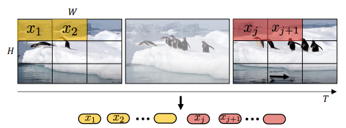
앞선 TimeSformer의 같은 경우 video clip을 transformer의 입력인 z로 embedding 하기 위해 프레임을 겹치지 않는 patch로 나눴습니다. 물론, temporal attention과 spatial attention을 같이 적용할지 따로 적용할지에 대해 실험을 하였지만 결국 사용하는 입력 patch는 한 프레임내의 NxN개와 총 프레임 수 t를 곱한 NxNxt개 였습니다. 이렇게 얻은 patch에 linear projection 시킬 수 있는 learnable matrix 곱 연산과 positional embedding이 더해져 transformer의 입력 z로 embedding 하였습니다. 이를 본 논문에서는 Uniform frame sampling 이라 소개합니다.
- Tubelet embedding
Uniform frame sampling의 경우 프레임 내의 patch를 얻을 땐 일정 크기의 너비(w) 및 높이(h)를 지닌 patch를 선정하였으나 시간 축으로의 크기가 항상 1이였습니다. 그러나 이 방식이외에 시간 축으로의 크기가 t인 tube 모양의 patch를 사용하는 방법 또한 도입하였으며 이를 Tubelet embedding이라 지칭하였습니다. 이와 같은 방식으로 나오는 patch의 수는 총 n_{h}*n_{w}*n_{t}개가 됩니다. Patch의 형태는 이해하기 쉽게 3D convolution의 kernel과 비슷한 형태라고 생각하시면 되겠습니다.
1.2 Transformer Models for Video
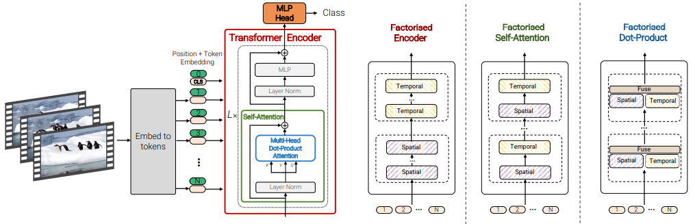
- Model 1 : Spatio-temporal attention
TimeSformer의 “Joint Space-Time” model와 동일한 모델 구조라하니 이전 리뷰를 참고해주시길 바랍니다.
- Model 2 : Factorised encoder
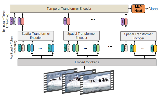
Model 2는 각 프레임마다 얻은 embedding z에 spatial attention을 각각 L_{s}번 반복해 프레임 개수만큼의 z^{L_{s}}를 얻고 이들을 모두 temporal attention의 입력으로 L_{t} 번의 attention을 반복하는 구조 입니다. Spatial attention을 마친 후, temporal attention을 적용하는 점에서 Image classification을 위한 ViT와 temporal attention이 만난 구조라 볼 수 있습니다. 이러한 방법을 통해 Model 1에 비해 learnable 파라미터 수는 늘었으나 복잡도가 (n_{h}*n_{w}*n_{t})^{2} 였던 것을 Model 2에서는 (n_{h}*n_{w})^{2} + n_{t}^{2} 로 줄여 연산량의 이점을 얻을 수 있다고 합니다.
- Model 3 : Factorised self-attention
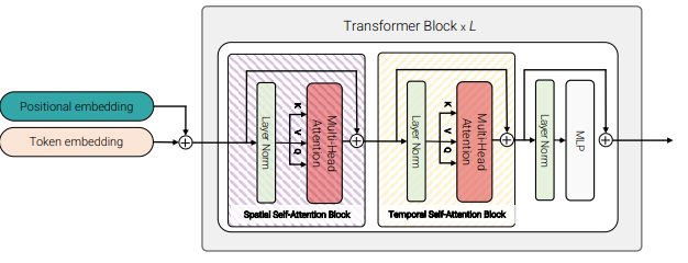
TimeSformer의 “Divided Space-Time” model와 동일한 모델 구조라하니 이전 리뷰를 참고해주시길 바랍니다. Model 2와 다른 점은 Model 2의 경우 spatial attention을 모두 마치고 temporal attention을 적용했다면 Model 3의 경우 Transformer block 내에 spatial attention 후 temporal attention을 적용하는 구조로 번갈아가며 적용된는 점 입니다.
- Model 4: Factorised dot-product attention
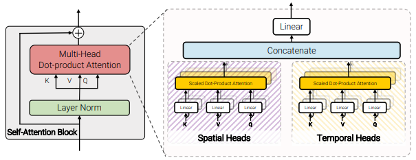
Model 4의 경우 한 Transformer block 내의 spatial attention이든 temporal attention이든 한번에 하나씩 Multi-Head Attention layer에 들어가 self-attention이 적용되었었는데 이를 깨고 Multi-Head Attention layer의 절반은 spatial attention 동시에 나머지 절반은 temporal attention을 적용한 뒤 embedding output을 concat하는 방식으로 하나의 block을 구성한 방법론입니다. 이와 같은 방식으로 구성해 Model 2, 3과 같은 연산 복잡도로 연산량의 이점을 가져가면서도, Model 1과 동일한 수의 learnable 파라미터를 지녀 용량에서도 이점을 지니게 되었습니다.
1.3 Initialisation by leveraging pretrained models
이전 TimeSformer를 소개드리면서 작성했다시피 Transformer 구조는 inductive bias가 약해 대용량 데이터 셋에서 장점을 보이며 이를 활용하기 위해서는 모델을 scratch부터 학습시켜야 합니다. 그러나 비디오 데이터 셋에 경우 이미지와 달리 비디오를 가리키는 하나의 label이 있다면 이를 가리키는 영상 데이터가 이미지의 수십~수백배는 더 많기에 현실적으로 scratch level 부터 학습 시키는 것은 상당히 어려운 문제 입니다. 이러한 이유로 본 논문에서는 기존 ViT 모델에서 아래 세가지 항목의 파라미터를 가져와 initial 파라미터로 사용하였다고 합니다.
- Positional embeddings : ViT의 positional embedding 파라미터를 프레임 개수만큼 t 번 반복시켜 같은 형태로 만든 뒤 initialize 하는 방식
- Embedding weights, E : Tubelet embedding 방식으로 patch를 이용해 embedding z를 만들때는 linear projection을 위한 learnable matrix가 3D 이기때문에 ViT의 linear projection matrix에서 “inflate” 방식으로 initalize 하는 방식, 추가적으로 time 축의 중간 프레임에서 사용되는 learnable matrix만 ViT의 linear projection matrix로 initalize하는 “central frame initialisation” 방식도 도입
- Transformer weights for Model 3 : 모델 구조 중 block 내의 spatial attention과 temporal attention이 동시에 있는 Model 3의 경우 spatial attention layer는 ViT로 initalize하고 temporal attention layer는 0으로 initialize
2. Experiments
실험에 앞서 하이퍼 파라미터에 따라 다음과 같이 명칭을 나누었습니다.
- ViT-Base (ViT-B) -> L=12, NH=12, d=3072
- ViT-Large (ViT-L) -> L=24, NH=16, d=4096
- ViT-Huge (ViT-H) -> L=32, NH=16, d=5120
L은 Transformer block 개수를 의미하며 NH는 block 내부 multi-head의 수, d는 multi-head의 output dimension을 의미합니다.
2.1 Input Encoding Methods
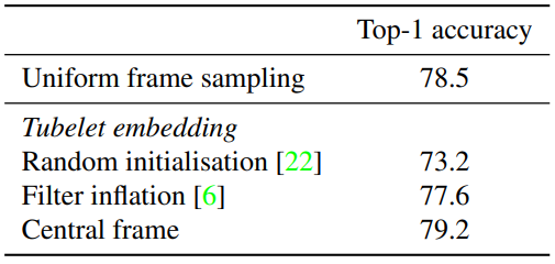
Table 1은 비디오를 embedding한 방식에 따른 성능입니다. Tubelet embedding의 경우 내부 파라미터의 initalize 방식에 따라 성능 차이가 큰 것을 알 수 있으며 Tubelet embedding을 Central frame 방식으로 initialize 하는 것이 가장 좋은 성능을 보여 이후 실험 모두를 이와 같은 방식을 사용해 initialize 하였다고 합니다.
2.2 Model Variants
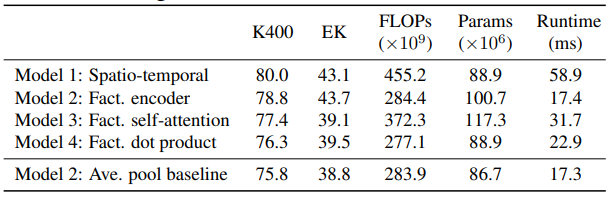
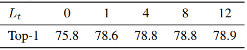
Table 2는 제안된 모델들의 Kinetics 400 데이터 셋에서의 성능 입니다. 베이스라인이 되는 Model 2에서 temporal attention 없이 spatial attention 받은 output을 averaging 하는 방법이 다른 제안된 모델들보다 가장 성능이 낮았으며 Model 1이 가장 높은 성능을 보여주었습니다. 이를 통해 temporal attention이 성능에 미치는 영향을 가늠해볼 수 있습니다. 그리고 Table 3의 경우 Model 2에서 temporal attention 횟수에 따른 성능을 보여줍니다. 횟수가 0일 경우 temporal attention 없이 spatial attention 받은 output을 averaging 하는 방법과 동일하며 일단 한번이라도 temporal attention을 적용하는 것이 성능 향상에 많은 영향을 끼지는 것을 알 수 있습니ㅏㄷ.
2.3 Comparison to state-of-the-art
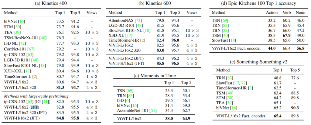
Table 4는 각 데이터 셋 별 ViViT의 성능 비교입니다. 크기가 큰 데이터 셋 Kinetics나 Moments in Time 의 경우 제안된 Model 1을 사용하였다고 하며 상대적으로 크기가 작은 데이터 셋 Epic Kitchens, SSv2 에서는 Model 2를 사용하였다고 합니다. TimeSformer와는 다르게 모든 데이터 셋에서 SOTA를 달성했으며 특히, JFT라는 대용량 데이터 셋으로 학습한 ViT의 파라미터를 이용해 transfer learning 했을때 다른 기존 방법론들과의 차이를 크게 보였습니다.
3. Reference
[1] https://arxiv.org/pdf/2103.15691.pdf