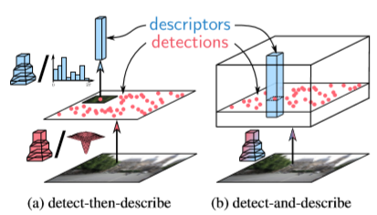
전통적으로 SIFT와 같은 알고리즘은 이미지에서 distinctive한 point를 “detect” 한 후 이 point들의 descriptor를 뽑는 “describe” 순서의 과정을 거쳤습니다.
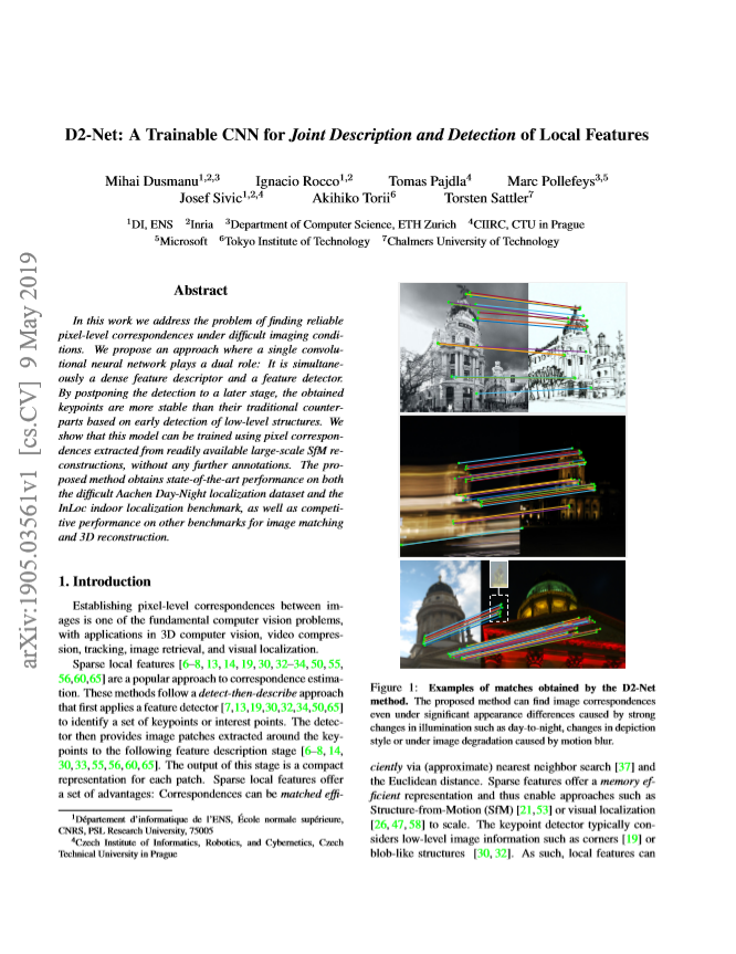
그러나 이러한 방법을 사용할 시, descriptor의 경우 large patch에서 high-level information (SIFT의 경우, gradient 방향과 크기에 대한 histogram) 을 사용하지만, detector의 경우 밤과 낮 같은 급격한 환경 변화가 있을 때 small patch에서 low-level information (edge, corner…) 의 변화로 불안정하다는 점이 있습니다.
그러나 reliable 하지 못한 detector와는 반대로 descriptor는 잘 매칭 시킨다는 것을 다른 논문이 리포팅한 점을 참고로 detector stage를 dense한 descriptor stage로 대체하여 한번에 “describe” 와 “detect” 순서로 계산하는 D2-Net을 설계했습니다.
1. Joint detection and description pipeline
1.1 Feature description
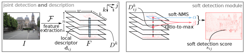
우선 이미지를 backbone network에 넣어 3D tensor F (feature)를 얻게 됩니다. 본 논문에서는 backbone network를 VGG16의 conv4_3까지 사용했습니다. 그리고 3D tensor F는 한 pixel의 n개의 channel로 묶었을 때 그 pixel을 설명해주는 descriptor vector라고 볼 수 있으며 이를 d로 나타낼 수 있게 됩니다.
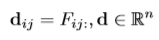
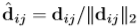
위 식에서 i는 이미지의 height 값이며, j는 width 값입니다.이 descriptor vector d는 Euclidean distance를 이용해 이미지 사이에 correspondence를 비교할 수 있게 해주는데, 저자는 비교하기 전에 L2 normalization을 적용했습니다.
1.2 Feature detection
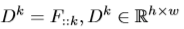
1.1에서는 한 pixel의 n개의 channel로 묶었다면 이번에는 n개의 channel을 하나씩 보게 됩니다. 3D tensor F 에서 각 channel, 즉 1차원의 h x w 의 feature map은 detection response map이라고 볼 수 있을 것이고 이는 해당 map 내 pixel마다의 score를 담고 있다고 볼 수 있을 것 입니다. 이는 SIFT에서의 DoG (Difference-of-Gaussians) 나 Harris’ corner detector에서 cornerness score map과 유사하지만, 이 논문에서는 이 response map에서 subset을 선택해 score를 후처리하게 됩니다. 제안된 detection 과정은 다음과 같이 두 부분으로 나뉩니다.
- Hard feature detection
SIFT의 DoG 에서는 해당 resolution의 앞뒤까지만 spatial non-local-maximum suppression을 적용하는 것에 반해, 3D tensor F는 SIFT의 octave에 비해 더 많은 n개의 channel이 있으며 이 중 어느 곳에서든 그 pixel을 대표할 수 있기 때문에 모든 channel을 보고 가장 큰 값을 가지고 있는 channel을 찾는 이 과정을 거치게 됩니다.
- Soft feature detection
Hard feature detection 후에 학습시 back-propagation을 위해 Soft feature detection 과정이 진행됩니다. 이 과정에서는 Fig 3.(right) 와 같이 soft detection score를 구하기 위한 두개의 파라미터 \alpha, \beta 를 구하게 됩니다.
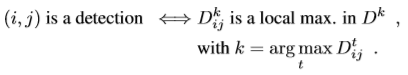
\alpha 는 다음과 같이 정의 되며 N은 (i, j)의 pixel 포함 주변 9개의 pixel의 집합으로 설정됩니다. 이 local softmax 연산은 hard feature detection에서 찾은 k인 channel에서 진행되며 다른 모든 pixel (decriptor) 에서도 이와 같은 ratio-to-max를 계산하게 됩니다.
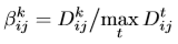
\beta 는 다음과 같이 정의되며 k번째의 channel의 feature map을 각 pixel 마다 channel-wise의 최대값을 나눠줍니다.
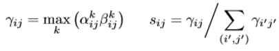
이렇게 구한 \alpha, \beta 중 pixel 마다 최대값을 선정하게되면 \gamma 라는 single score map을 얻게됩니다. 그리고 이를 normalize 하여 soft detection score s를 얻게 됩니다.
- Multiscale detection
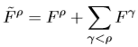
주로 CNN network를 학습을 할 때 scale invariant한 data augmentation을 하기도 하는데 이는 주로 다른 view-point로 물체를 봤을 때 miss match 되는 경향이 있다. 이러한 경향에 불변하기 위해 inference 에서 적용되는 image pyramid 기법을 사용합니다. Pyramid는 resolution이 원래 이미지의 \rho=0.5, 1, 2배가 되는 I^{ \rho } 를 이용하며 feature map F^{ \rho} 를 구하게 되고 low resolution feature map을 high resolution feature map에 detection을 누적하여 구하게 됩니다. 만약 같은 영역을 detect 했다면 lower feature map의 detection을 선택하게 됩니다.
2. Jointly optimizing detection and description
2.1 Training loss
학습시 network가 view-point가 바뀌는 등의 변화가 있는 상황에서도 repeatable하게 detect 되게 하고, corresponding point를 잘 찾을 수 있는 distinctive 한 descriptor를 가지게 하기 위해 triplet margin ranking loss를 사용했습니다. Triplet margin ranking loss는 triplet loss와 유사하며 다음과 같은 수식으로 정의됩니다.

여기서 p(c)는 두 이미지 사이의 corresponding point 간 distance를 줄이기 위한 positive descriptor distance 이며 아래와 같습니다.
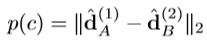
A와 B는 각각 이미지 쌍 (I_{1}, I_{2}) 의 corresponding point이며 \widehat{d}^{(1)}_{A}, \widehat{d}^{(2)}_{B} 는 각 이미지의 corresponding descriptor 입니다.
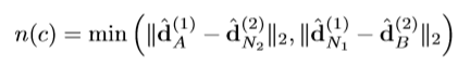
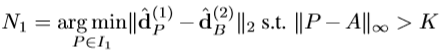
그리고 n(c)는 각 이미지의 corresponding point와 negative 사이의 distance를 늘리기 위한 negative descriptor distance 이며 위와 같습니다. Negative는 \widehat{d}^{(1)}_{A}, \widehat{d}^{(2)}_{B} 의 hardest negative를 선정하며 아래와 같고 N2도 같은 방식으로 찾게 됩니다.
이렇게 정의된 loss는 descriptor의 distinctiveness를 강화하도록 학습하게 되며 detection의 repeatability 를 강화하기 위해 detection term을 추가해 weight를 주며 최종적으로 아래와 같은 loss를 줄이도록 학습하게 됩니다.
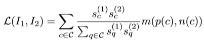
{s}^{(1)}_{c}과 {s}^{(2)}_{c} 는 각각 I_{1}, I_{2} 의 soft detection score 이며 C는 I_{1}, I_{2} 사이의 모든 corresponding point들의 집합입니다.
Result
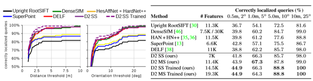
제안된 D2-Net은 Fig 4. 에서 보다시피 Aachen Day-Night dataset에서 DELF보다 높은 성능으로 state-of-the-art를 달성 했습니다. 이외에도 다른 실험을 많이 하였으니 자세한 사항은 논문을 참고해 주시기 바랍니다.